How Four Numbers Can Paint a Nebula
At first glance, the images look like deep-space photography—vast, swirling nebulae of violet, electric blue, and gold. But these cosmic clouds weren't captured by the James Webb Space Telescope. They were "found" inside four simple numbers and a pair of trigonometry functions.
This is the world of the Peter de Jong attractor, a mathematical engine that turns simple recursion into infinite complexity.
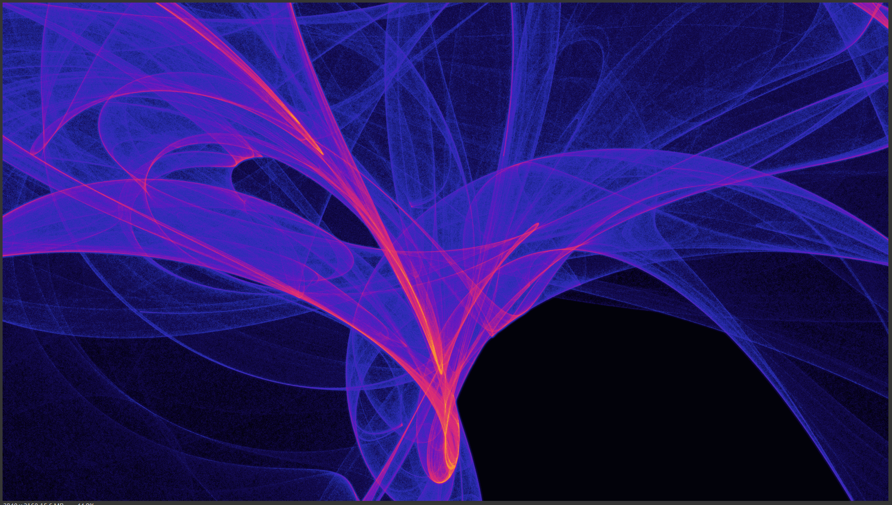
A raw Peter de Jong attractor rendered with ten million points. Look at the way the deep indigo ribbons weave across the frame like gossamer silk, eventually converging into a heart-shaped nexus that glows with a fiery, ember-like intensity. The "glow" is not painted; it is the physical density of a mathematical path.
The Peter de Jong Engine
The math behind the first image is deceptively simple. It follows two equations that update the position of a point (x,y) over and over:
xn+1=sin(a⋅yn)−cos(b⋅xn)
yn+1=sin(c⋅xn)−cos(d⋅yn)
With just four constants—a,b,c,d—we can generate a "strange attractor." If you plot only a few thousand points, you see nothing but noise. But as you climb into the millions, a "ghost" begins to emerge. Some regions of the coordinate plane are visited more often than others, creating the structure you see. The final render comes from mapping this density to a vivid color gradient, where the most visited points glow white-hot.
The Golden Spiral Twist
While the raw attractor is beautiful in its chaotic symmetry, we can push the math further by introducing one of nature’s favorite constants: PHI (ϕ), or the Golden Ratio (~1.618).
By taking the coordinates from the De Jong attractor and wrapping them around a logarithmic spiral, we evoke the same geometry found in sunflower seeds, nautilus shells, and hurricane arms.
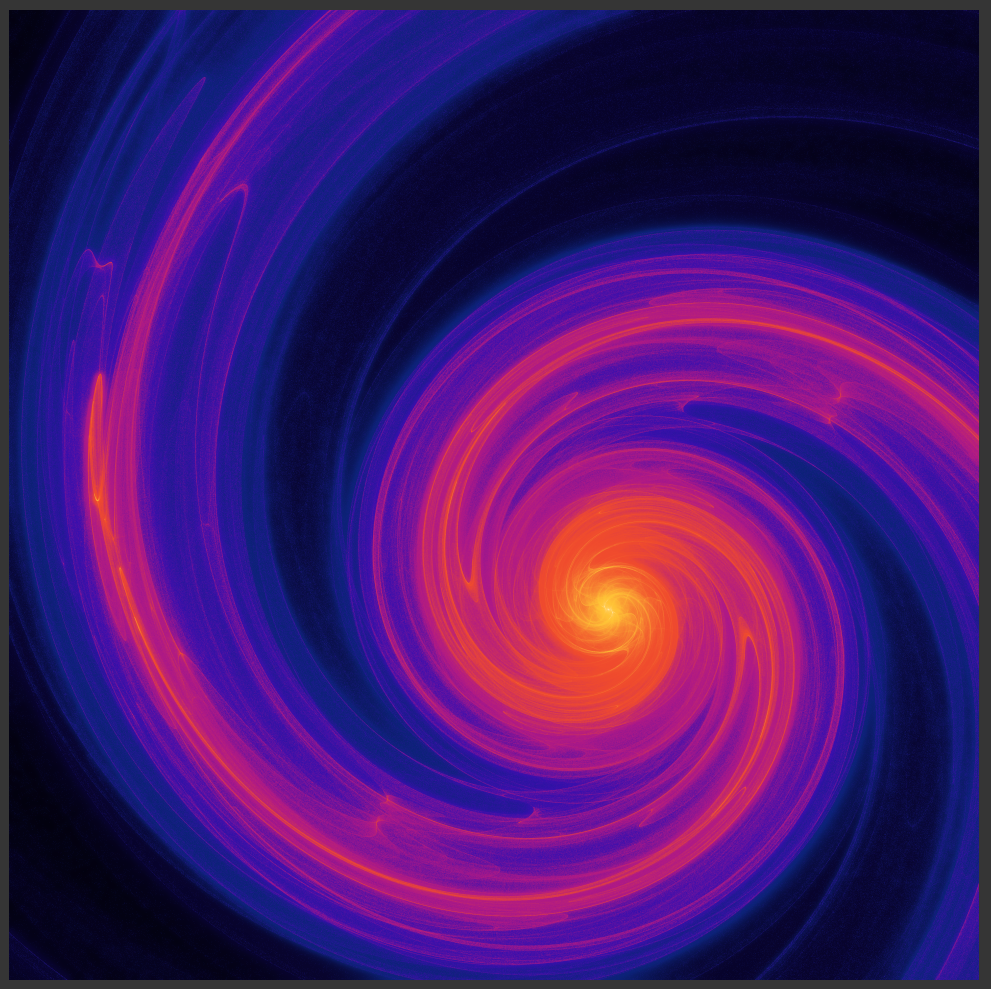
The intersection of chaos and order: A De Jong attractor mapped onto a Golden Spiral (ϕ).
By mapping the "chaotic" output of the attractor onto the "ordered" growth of the spiral, the artwork takes on a more organic, biological feel. It stops looking like a digital glitch and starts looking like a galaxy.
One of the most beautiful aspects of this math is that changing the parameters a,b,c,d even slightly results in completely different images. It is a testament to the beauty of math and chaos: infinite variety from a single, simple seed.
From Math to Light
The secret to the "photographic" quality of these images isn't just the math—it's the tone mapping.
In the real world, light doesn't behave linearly. If you double the number of points in a pixel, it doesn't necessarily look "twice as bright" to the human eye. To capture the wispy, ethereal edges of the nebula, the algorithm uses a Logarithmic Scale and Gamma Correction. This "stretches" the data, allowing us to see the faint, single-point trails as clearly as the dense, million-point clusters.
As the Wolfram MathWorld documentation on attractors notes, these systems are "strange" because they have fractal dimensions. They are infinite detail packed into a finite space.
A Universe in a Script
There is a certain poetry in the fact that the logic for these images is less than 150 lines of code. It proves that you don't need a brush to paint a masterpiece—sometimes, you just need a very good set of coordinates.
Next time you look at a spiral or a storm, remember the four numbers. They might be the only thing standing between us and the void.
View the Python Code
The Chaos Engine (De Jong Attractor)
import numpy as np
from PIL import Image
from scipy.ndimage import gaussian_filter


def dejong_chaos(W=1920, H=1080, iters=50_000_000, burn=10_000,
                 a=1.4, b=-2.3, c=2.4, d=-2.1,
                 seed=0, out="dejong_chaos.png"):
    rng = np.random.default_rng(seed)

    # --- Render at 2x for supersampling, then downscale ---
    SW, SH = W * 2, H * 2

    # Burn-in phase (scalar, short)
    x, y = rng.uniform(-0.1, 0.1), rng.uniform(-0.1, 0.1)
    for _ in range(burn):
        x, y = np.sin(a * y) - np.cos(b * x), np.sin(c * x) - np.cos(d * y)

    # Vectorized iteration in large batches
    hist = np.zeros((SH, SW), dtype=np.float64)
    scale = 0.45
    batch = 500_000
    remaining = iters - burn

    while remaining > 0:
        n = min(batch, remaining)
        xs = np.empty(n, dtype=np.float64)
        ys = np.empty(n, dtype=np.float64)
        cx, cy = x, y
        for i in range(n):
            cx, cy = np.sin(a * cy) - np.cos(b * cx), np.sin(c * cx) - np.cos(d * cy)
            xs[i] = cx
            ys[i] = cy
        x, y = cx, cy

        px = ((xs * scale + 0.5) * (SW - 1)).astype(np.int32)
        py = ((ys * scale + 0.5) * (SH - 1)).astype(np.int32)
        mask = (px >= 0) & (px < SW) & (py >= 0) & (py < SH)
        np.add.at(hist, (py[mask], px[mask]), 1.0)
        remaining -= n
        print(f"  {iters - remaining:,} / {iters:,} points computed")

    # --- Multi-layer glow for nebula bloom ---
    glow_fine = gaussian_filter(hist, sigma=2.0)
    glow_wide = gaussian_filter(hist, sigma=8.0)
    hist = hist + glow_fine * 0.4 + glow_wide * 0.25

    # --- Tone mapping: log + aggressive gamma to spread values ---
    img = np.log1p(hist)
    img = img / (img.max() + 1e-9)
    img = np.power(img, 0.55)  # strong gamma lift: pushes wisps into vivid range

    t = img  # [0,1]

    # --- 7-stop vivid color gradient ---
    #  black -> deep indigo -> electric blue -> violet -> hot pink -> gold -> white
    stops = np.array([
        [2,    2,   10],     # near-black
        [15,   5,   60],     # deep indigo
        [20,   60,  180],    # electric blue
        [100,  20,  200],    # violet
        [220,  40,  120],    # hot pink
        [255,  170,  30],    # gold / amber
        [255,  252,  240],   # warm white
    ], dtype=np.float32)
    edges = [0.0, 0.08, 0.22, 0.40, 0.58, 0.80, 1.0]

    rgb = np.zeros((SH, SW, 3), dtype=np.float32)
    for i in range(len(edges) - 1):
        lo, hi = edges[i], edges[i + 1]
        mask = (t >= lo) & (t < hi) if i < len(edges) - 2 else (t >= lo)
        frac = np.clip((t - lo) / (hi - lo), 0, 1)
        # smooth-step interpolation for silkier color transitions
        frac = frac * frac * (3 - 2 * frac)
        blend = stops[i] * (1 - frac[..., None]) + stops[i + 1] * frac[..., None]
        rgb[mask] = blend[mask]

    # --- Downsample from 2x supersampled to final resolution ---
    rgb8 = np.clip(rgb, 0, 255).astype(np.uint8)
    full = Image.fromarray(rgb8)
    final = full.resize((W, H), Image.LANCZOS)
    final.save(out, quality=95)
    print(f"Saved {out} ({W}x{H})")
    return out


dejong_chaos(W=2*1920, H=2*1080, iters=10_000_000,
             a=1.4, b=-2.3, c=2.4, d=-2.1, out="chaos_spark.png")
The Golden Spiral Mapping
import numpy as np
from PIL import Image
from scipy.ndimage import gaussian_filter

PHI = (1 + np.sqrt(5)) / 2


def dejong_golden_spiral(W=480, H=270, iters=1_000_000, burn=5_000,
                         a=1.4, b=-2.3, c=2.4, d=-2.1,
                         seed=42, out="chaos3.png"):
    rng = np.random.default_rng(seed)

    hist = np.zeros((H, W), dtype=np.float64)

    b_sp = 2.0 / np.pi * np.log(PHI)
    a_sp = min(W, H) * 0.010
    # Golden ratio positioning: focal point at (1/PHI, 1/PHI) from edges
    # matching the reference image where the spiral coils into the
    # lower-right golden intersection point
    cx = W * (1.0 / PHI)       # ≈ 0.618 from left
    cy = H * (1.0 / PHI)       # ≈ 0.618 from top

    max_theta = 8 * np.pi
    arm_width = min(W, H) * 0.04

    # Two spiral arms offset by π (like a galaxy)
    arm_offsets = [0.0, np.pi]

    # Layers: tight core → wispy outer haze
    layers = [
        # (da, db, dc, dd, weight, ang_jitter, rad_scale)
        (0,      0,      0,      0,      1.0,  0.25,  1.0),
        (+0.3,  -0.5,   +0.2,   +0.4,   0.7,  0.45,  1.3),
        (-0.2,  +0.7,   -0.3,   -0.6,   0.5,  0.70,  1.8),
        (+0.8,  +0.3,   -0.5,   +0.9,   0.4,  1.00,  2.5),
        (-0.5,  -0.8,   +0.6,   -0.3,   0.3,  1.40,  3.5),
    ]

    plotted = 0
    print("Iterating attractor → spiral mapping...")
    for li, (da, db, dc, dd, weight, ang_jit, rad_sc) in enumerate(layers):
        la, lb, lc, ld = a + da, b + db, c + dc, d + dd

        # Different seed per layer for variety
        lrng = np.random.default_rng(seed + li * 137)
        lx, ly = lrng.uniform(-0.1, 0.1), lrng.uniform(-0.1, 0.1)
        for _ in range(burn):
            lx, ly = np.sin(la * ly) - np.cos(lb * lx), np.sin(lc * lx) - np.cos(ld * ly)

        layer_iters = int(iters * weight)
        for i in range(layer_iters):
            lx, ly = np.sin(la * ly) - np.cos(lb * lx), np.sin(lc * lx) - np.cos(ld * ly)

            theta_base = ((lx + 2.0) / 4.0) * max_theta + (ly * ang_jit)
            r_spiral_base = a_sp * np.exp(b_sp * theta_base)
            radial_offset = (ly / 2.0) * arm_width * rad_sc * (1.0 + r_spiral_base / (min(W, H) * 0.4))

            # Plot on both spiral arms
            for arm_off in arm_offsets:
                theta = theta_base + arm_off
                r_spiral = a_sp * np.exp(b_sp * theta_base)  # radius stays same
                r_total = r_spiral + radial_offset

                px_f = cx + r_total * np.cos(theta)
                py_f = cy + r_total * np.sin(theta)
                px_i = int(px_f)
                py_i = int(py_f)

                if 0 <= px_i < W and 0 <= py_i < H:
                    hist[py_i, px_i] += weight
                    plotted += 1

        print(f"  layer {li} w={weight} jit={ang_jit}: {layer_iters:,} done")

    print(f"  Plotted {plotted:,} points")

    # --- Multi-layer glow ---
    s = max(1.0, min(W, H) / 270.0)
    glow_fine = gaussian_filter(hist, sigma=0.8 * s)
    glow_mid  = gaussian_filter(hist, sigma=2.5 * s)
    glow_wide = gaussian_filter(hist, sigma=7.0 * s)
    hist = hist + glow_fine * 0.5 + glow_mid * 0.3 + glow_wide * 0.2

    # --- Tone mapping ---
    img = np.log1p(hist)
    img = img / (img.max() + 1e-9)
    img = np.power(img, 0.48)

    t = img

    # --- 8-stop cosmic nebula gradient ---
    stops = np.array([
        [1,    1,    5],      # void
        [8,    4,   45],      # deep indigo
        [12,  35,  120],      # dark sapphire
        [55,  15,  175],      # deep violet
        [175, 25,  135],      # magenta
        [240, 75,   45],      # ember
        [255, 195,  55],      # gold
        [255, 248, 225],      # warm white
    ], dtype=np.float32)
    edges = [0.0, 0.05, 0.14, 0.28, 0.44, 0.60, 0.80, 1.0]

    rgb = np.zeros((H, W, 3), dtype=np.float32)
    for i in range(len(edges) - 1):
        lo, hi = edges[i], edges[i + 1]
        mask = (t >= lo) & (t < hi) if i < len(edges) - 2 else (t >= lo)
        frac = np.clip((t - lo) / (hi - lo), 0, 1)
        frac = frac * frac * (3 - 2 * frac)
        blend = stops[i] * (1 - frac[..., None]) + stops[i + 1] * frac[..., None]
        rgb[mask] = blend[mask]

    rgb8 = np.clip(rgb, 0, 255).astype(np.uint8)
    Image.fromarray(rgb8).save(out, quality=95)
    print(f"Saved {out} ({W}x{H})")
    return out


dejong_golden_spiral(W=8*480, H=8*480, iters=10_000_000, burn=5_000,
                     a=1.4, b=-2.3, c=2.4, d=-2.1,
                     seed=42, out="chaos_golden.png")